One Number Is Rarely Enough
Why prediction intervals are critical (and challenging!) for HR predictive analytics
This article is the first in a three-part series on “Advanced modelling of workers’ future performance ranges through ANNs with custom loss functions.” Part 1 explores why it’s useful to predict the probable ceiling and floor for an employee’s future performance — and why it’s difficult to do so effectively, using conventional methods based on mean absolute error or standard deviation. Part 2 investigates how one can model the likely ceiling and floor using separate artificial neural networks with custom loss functions. And Part 3 combines those ceiling and floor models to create a composite prediction interval that can outperform simpler models based on MAE or SD in forecasting the probable range of workers’ future job performance.
Why it’s useful to predict the range of a worker’s likely future performance
Imagine that you’re the Director of Production in a manufacturing plant, and you’re planning the work to be carried out tomorrow by your employees. You’ve received a production order from a critical client for 1,600 units that absolutely must be completed by the end of the day tomorrow, and you only have one milling machine capable of producing the units — so you can’t split the assignment between multiple workstations. Rather, you’ll need to choose the one machine operator whom you believe is most likely to achieve the target and then give that person the freedom to work.
Thankfully, you have a robust predictive analytics system in place that integrates data from various OEE, ERP, and HRM tools, and for each of the 50 machine operators in your factory, the system is capable of generating a prediction of how many units each person would be likely to produce tomorrow, if he or she were assigned to the milling machine. From among all the candidates, the system predicts that there are just two machine operators (“Worker A” and “Worker B”) who would be expected to meet the necessary target, if assigned to the relevant machine tomorrow — and that they have an identical predicted output:
Predicted output on the milling machine tomorrow:
Worker A: 1,620.5 units
Worker B: 1,620.5 units
Worker C: 1,530.0 units
Worker D: 1,490.5 units
Based on that information — and in the absence of any other experience, insights, or intuitions on the part of your managers that might point toward one worker or the other — you might be inclined to pick randomly between Workers A and B. The system’s predictive analytics haven’t yet identified any factors that would allow it to offer useful prescriptive analytics.
In reality, though, your analytics system may contain additional information that could aid you in making that decision — even if it’s not (yet) explicitly sharing it with you. For example, when the system states that a given person is likely to produce “1,620.5 units” if assigned to the milling machine tomorrow, what it may actually be telling you is, “I ran a single predictive model which determined that the number of units produced by this person tomorrow is likely to be between 1,464.7 and 1,776.3, and 1,620.5 is the midpoint of that range,” or “I ran five different predictive models, each of which generated a different projected value (the lowest of which was 1,358.9 and the highest of which was 1,805.4), and 1,620.5 is the average of all five of their predictions.”
Along those lines, imagine that the system were to explicitly present you with this information:
Predicted output on the milling machine tomorrow:
Worker A: 1,620.5 units (likely range: 1,493.5 – 1,747.5)
Worker B: 1,620.5 units (likely range: 1,608.5 – 1,632.5)
By offering this additional information, your analytics system is now performing an important prescriptive role. Assuming that you’ve found the system’s predictions to be generally reliable in the past, you have clear grounds for choosing to assign the critical order to Worker B rather than Worker A. It’s true that Worker A has a realistic potential of producing 1,700 units tomorrow, which significantly exceeds Worker B’s potential ceiling. But that’s not particularly meaningful or helpful. The only thing you’re really concerned with is that at least 1,600 units get produced tomorrow, so you can fill your client’s order — and from that perspective, assigning the task to Worker A is quite risky, as there’s a significant chance that he or she will fall far short of that goal. While having the exact same predicted output of 1,620.5 units, Worker B’s predicted performance covers a much narrower range: even if he or she has a bad day tomorrow (or the model’s prediction interval for both workers turns out to have been a bit too optimistic), Worker B still seems likely to hit the necessary target.
We can thus see why it’s helpful to forecast not only the single continuous value that represents our best estimate of a worker’s actual future performance but also the likely “ceiling” and “floor” for that worker’s performance. (Indeed, in some cases, we may not even be interested in trying to pinpoint the likely “target value” at all: as managers, the predicted ceiling and predicted floor may themselves give us all the information that we need in order to make critical decisions.) So how can we go about predicting the probable range of a worker’s future performance?
Simple approaches to indicating probable performance ranges
Imagine that you’ve developed a machine-learning model for your factory that’s capable of predicting a worker’s mean daily efficacy during the next 30 days. By validating the model on historical data, you’re able to compare the model’s predicted target efficacy values with the actual mean efficacy values that workers ultimately displayed during the relevant 30 days. To illustrate this scenario, we’ll use synthetic data that was generated with the open-source Synaptans WorkforceSim package (a Python-based platform) and a Random Forest model that was created with the Comport_AI package (another open-source Python web app). The synthetic dataset simulated the daily behaviors of a factory’s workforce of 268 persons over a period of 300 days. Below we can see the results of the “Base Target Model” whose Random Forest algorithm generated predictions for workers’ mean efficacy during the next 30 days.

During the process of model training and validation (or during the inference process itself), such machine-learning models generate a wealth of data that can be exploited to give a predictive analytics system’s user some sense of the “range” within which a worker’s future performance is likely to fall. There are various approaches to conceptualizing such a range, each of which conveys different information to a system’s user.
Mean absolute error of a model
One simple approach is to simply report the mean absolute error (MAE) demonstrated by a system’s predictive model during its training and validation process. A model’s MAE can be calculated by finding the absolute difference between the actual and predicted value for each observation, taking the sum of those absolute differences for all observations, and dividing them by the number of observations. It’s represented by the formula:

In our case, y might be a single actual future efficacy score for a worker, p the predicted future efficacy score for the given period that was produced by a model, and n the total number of worker-periods for which predictions were generated. Employing such an approach, imagine that you’ve trained and validated two Random Forest models using slightly different hyperparameters, and the models have generated the following forecasts regarding two of your employees, Workers E and F:
Prediction made using Model 1
Worker E’s predicted efficacy during next 30 days: 85.73
Mean absolute error of Model 1: 3.18

Prediction made using Model 2
Worker F’s predicted efficacy during next 30 days: 85.73
Mean absolute error of Model 2: 35.72
This suggests that Worker E’s efficacy during the next 30 days (which was produced with the aid of Model 1) is indeed likely to be quite close to 85.73, whereas Worker F’s efficacy (predicted by Model 2) could easily be dramatically higher or lower than 85.73. This isn’t because Worker F is inherently any less “stable” or “reliable” than Worker E, but simply because Model 1 is able to make predictions with a much lower degree of error than Model 2.
The image below (which draws on the Base Target Model produced by Comport_AI) visually illustrates the kind of “prediction interval” that we get when we take the predicted target value generated for each worker and then add the model’s MAE to the predicted target value (to obtain the predicted ceiling value) and subtract the model’s MAE from the predicted target value (to obtain the predicted floor value). Here the black dots within the green area represent actual target values that fell within the predicted ceiling-floor range, while black dots in the pink areas reflect actual target values that fell outside of the predicted range.

We immediately notice that such a simple MAE-based prediction interval is characterized by the fact that (1) the size of the prediction interval is the same for every worker-period and (2) a large number of actual target values either exceeded the predicted ceiling value or fell below the predicted floor value.
Standard deviation of a worker’s past performance
Mean absolute error gives a sense of how errant a model’s predictions are on the whole, for the entire community of workers. But a prediction interval based on a model’s MAE is unable to take advantage of the reality that — in principle — it should be possible to predict future performance with a narrower window for workers who have historically shown themselves to be highly consistent and reliable, even if a model is only capable of offering a broader “guess” regarding the future performance of workers whose behavior has been highly variable and inconsistent from day to day.
With that possibility in mind, another potential approach to performance-range modelling is to incorporate the predicted target efficacy value that a worker is expected to demonstrate during the next 30 days, along with the (population) standard deviation of the efficacy values that the worker has displayed in the past. This standard deviation can be calculated as:

Here x is a single actual daily efficacy score for the worker, µ is the worker’s mean efficacy across all days, and n is the number of days for which the worker has efficacy scores. Building a performance-range model in this manner will allow us to keep the prediction interval small for as many workers as possible, while allowing it to expand for others (as necessary).
Using our Base Target Model generated in Comport_AI, we can see what such prediction intervals look like when they’re produced by calculating (1) predicted target values ± 1.0×SD and (2) predicted target values ± 0.8×SD.

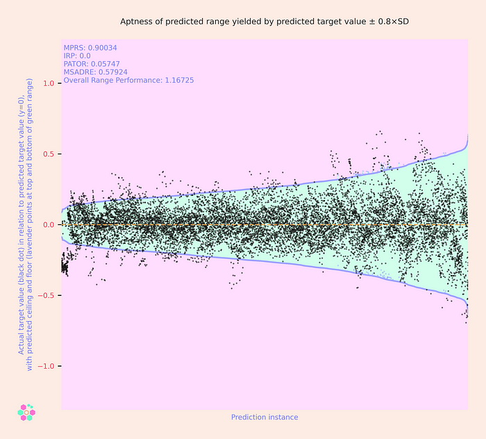
Here we see that in comparison to the MAE-based prediction intervals, SD-based prediction intervals are much more flexible. If we set the multiplier high enough (e.g., at 1.0), the SD-based prediction intervals are large enough to include the overwhelming majority of actual target values — but at the cost of having intervals that, in most cases, were unnecessarily large. Decreasing the SD multiplier (e.g., to 0.8) reduces the size of the prediction intervals — potentially rendering them more useful as a tool for making managerial decisions — while at the same time causing more actual target values to fall outside of the predicted range (which is not helpful).
While such an SD-based approach has some advantages, it’s less than dependable as a tool for gauging the size of the range that represents how much an actual future value is likely to differ from the predicted value. In itself, the standard deviation of a worker’s past performance values doesn’t directly provide us with any indication regarding how wide or narrow the prediction interval for a worker’s projected future performance is. For example, to switch (for the moment) from our 30-day forecasts to the prediction of workers’ behavior tomorrow, consider a scenario in which a hypothetical Worker G has always historically displayed exactly the following pattern of daily efficacy:
Efficacy on Mondays: 48.0
Efficacy on Tuesdays: 49.0
Efficacy on Wednesdays: 50.0
Efficacy on Thursdays: 51.0
Efficacy on Fridays: 52.0
Meanwhile, a hypothetical Worker H has always exactly displayed the following pattern:
Efficacy on Mondays: 10.0
Efficacy on Tuesdays: 90.0
Efficacy on Wednesdays: 30.0
Efficacy on Thursdays: 70.0
Efficacy on Fridays: 50.0
Here, Worker G’s daily efficacy has a standard deviation of ≈1.41, while Worker H’s has a standard deviation of ≈28.28. Now imagine that tomorrow will be Thursday, and your predictive analytics system outputs the following projections:
Worker G’s predicted efficacy tomorrow: 51.0
SD of Worker G’s daily efficacy values: 1.4142

Worker H’s predicted efficacy tomorrow: 70.0
SD of Worker H’s daily efficacy values: 28.2843
When analyzing the historical population of efficacy scores that have already been collected for a given worker, we can say that a randomly selected score will fall within 1 SD above or below the mean in roughly 68.3% of cases and within 2 SDs of the mean in roughly 95.5% of cases. For example, roughly 68.3% of Worker H’s past efficacy scores fell within a distance of 28.28 from his or her mean historical score, while 68.3% of Worker G’s past efficacy scores fell within the much narrower range of just 1.41 above or below his mean historical score. This might seem to suggest that we’re in a position to make more “accurate” forecasts regarding Worker G’s future efficacy than Worker H’s.
In reality, though, the picture is more complicated — and it would be unsound to interpret the standard deviation as if it were directly indicating the distance from the predicted values within which the actual values are likely to fall in a certain number of cases.
The role of (optimized) prediction intervals
To help us explore this fact, we can use the term “optimized prediction interval” to refer to the forecasted range within which a machine-learning model says that some actual future value is likely to fall. Sometimes the term “prediction interval” is used in a narrow sense to refer to a type of range that’s represented by the formula [µ — zσ, µ + zσ], where µ reflects the mean of a population, σ its standard deviation, and z a factor related to whether one hopes for 90% (z ≈ 1.64), 95% (z ≈ 1.96), or some other percentage of actual values to fall within the calculated distance from the predicted values in the given percentage of cases. (The related “prediction bands” are calculated on the basis of such prediction intervals.) For our purposes, we’ll thus use the term “optimized prediction interval” to emphasize the fact that we’re not limiting ourselves to the sort of prediction interval that’s calculated using standard deviation; rather, we want to find the best possible estimate of the range within which an actual value is likely to fall — regardless of whether it can be calculated using SD or needs to be determined through some other, more sophisticated means.
If a larger standard deviation in past performance directly entailed a larger optimized prediction interval for tomorrow’s performance, it would be reasonable to expect that Worker G’s efficacy tomorrow will indeed be quite close to 51.0 — but that Worker H’s efficacy might be wildly higher or lower than 70.0. But in reality, a higher historical SD doesn’t necessarily translate to a less reliable forecast. We would expect any good predictive analytics system that has access to the relevant data to be just as successful at predicting Worker H’s efficacy tomorrow as at predicting Worker G’s — because both employees have unfailingly demonstrated a pattern of performance that’s easily “learnable,” despite the superficially more variable and erratic performance of Worker H.
Nevertheless, while it’s not mathematically necessary that larger standard deviations will translate to larger optimized prediction intervals (and lower forecast quality), as a practical matter, the two are often linked. In the real world, workers don’t follow such predictable clockwork patterns as Workers G and H — and if a person displayed such huge daily swings in performance as Worker H, it would indeed be difficult for any model to uncover a perfectly discernible pattern in that data. Such huge variations are more likely to indicate a degree of (unpredictable) randomness than a perfectly deterministic and predictable (but incredibly complex) pattern. In practice, even good models will typically generate less confident predictions and a larger optimized prediction interval for someone like Worker H.
“But my workers’ behavior isn’t normal!”
Approaches like the ones based on MAE and SD that we’ve discussed above have a number of limitations. Among them is fact that they presume that both halves of an optimized prediction interval (i.e., the “top” and “bottom”) will be symmetrical. In other words, if a given model predicts that a worker will have an efficacy of 84.0 tomorrow, it’s equally probable that the person’s actual efficacy will be higher than that number as that it will be lower than it, and the actual figure is just as likely to be, say (84.0–1.0) = 83.0 as it is to be (84.0 + 1.0) = 85.0.
But in the kinds of forecasting scenarios that HR predictive analytics deals with, such symmetry often doesn’t exist: data relating to workers’ performance frequently displays a skewed or other non-normal distribution, and employing machine-learning models and formulas that presume a normal distribution (or standard “bell curve”) can yield predictions that have an unnecessarily high degree of error.
For example, imagine that a model’s best prediction is that a given machine operator will have an efficacy of 98.3% tomorrow. Assuming that the machines and metrics have been properly calibrated, 100.0% (or something just slightly above 100%) represents the highest possible efficacy score that a worker could possibly achieve on that machine. After all, if an assembly line’s conveyor belt has a fixed speed, that establishes a hard maximum on the number of units that can be produced by a single person in a given eight-hour period. So while it might be possible for the operator to record an actual efficacy of 98.5%, or 99.2%, or even 100.6% tomorrow, it’s not possible for him or her to record an actual efficacy of 148.3% (or 50 pp. higher than the prediction). However, it is certainly possible for the operator to record an actual efficacy of 48.3% (or 50 pp. lower than the prediction), if tomorrow the machine were to suffer a series of severe mechanical failures, each of which required the operator to devote significant time to repairing and restarting the device. It isn’t possible to fully capture the reality of that situation by choosing a single number to represent the midpoint of the optimized prediction interval and then forecasting, for example, that the worker has a projected efficacy for tomorrow of “98.3% ± 5.3 pp.” or “98.3% ± 8.1 pp.”
Similarly, imagine that a predictive analytics system forecasts that a given employee is likely to have 0.93 absences during the next 30 days. The only way the actual figure could turn out to be lower than the target is if the worker has zero absences; it’s not possible for a worker to have -2 or -5 absences. But the range of potential actual outcomes on the other side of the predicted value is much wider: the worker might have 1, 2, 5, or even 10 absences during the next month. A predictive analytics system for HR that forecasts that a given worker’s number of absences during the next 30 days will be, say, “0.93 ± 2.4” is likely to simply confuse users. How would one even go about interpreting such a prediction?
Can we do better?
The good news is that there are alternative approaches to predicting the likely range of a worker’s future performance that — while somewhat more complex — have the potential to generate more accurate, nuanced, and useful predictions. In Part 2 of this series, we’ll investigate how more realistic and meaningful predicted performance ranges can be generated using machine learning that that seeks to separately model (1) the likely ceiling for a worker’s future performance and (2) the likely floor for the worker’s future performance, with the aid of artificial neural networks whose custom loss functions help them learn to create performance intervals that are as small as possible, while still being just large enough to include the actual future value that the worker will display in the greatest possible majority of cases. I hope that you’ll join us for Part 2 of the series!
