A Better Way of Forecasting Employees’ Performance
Evaluating the use of composite ceiling-floor models for predicting the likely range of workers’ future job performance
This article is the third in a three-part series on “Advanced modelling of workers’ future performance ranges through ANNs with custom loss functions.” Part 1 explored why it’s useful to predict the probable ceiling and floor for an employee’s future performance — and why it’s difficult to do so effectively, using conventional methods based on mean absolute error or standard deviation. Part 2 investigated how one can model the likely ceiling and floor using separate artificial neural networks with custom loss functions. And Part 3 combines those ceiling and floor models to create a composite prediction interval that can outperform simpler models based on MAE or SD in forecasting the probable range of workers’ future job performance.
Building joint range models
In our effort to develop more effective means for predicting the range within which a worker’s future performance will likely fall, we’ve seen how one artificial neural network with a custom loss function can learn to predict a range’s ceiling more successfully than conventional MAE- or SD-based methods, while another ANN with a different custom loss function learns to better predict its floor. But our ultimate goal isn’t to predict just a floor or ceiling; it’s to forecast the range of a worker’s likely future performance, which is a single prediction interval bounded by a floor and ceiling.
To that end, in this final part of our series, we’ll combine particular ceiling models that we developed in Part 2 with particular floor models, to create what we can refer to as “joint range models.” For each predicted target value (i.e., the Base Target Model’s best estimate of the mean efficacy that a given worker will display during the next 30 days), the joint range model will generate a prediction interval that’s defined by its predicted ceiling and predicted floor and that includes the predicted target value somewhere within its interior. It’s important to note that while simpler MAE- or SD-based models will generate prediction intervals that have the predicted target value located precisely at the midpoint between ceiling and floor (except in cases where the floor has been artificially prevented from being less than zero), the more advanced ANN-based ceiling and floor models that we developed in Part 2 are capable of yielding more nuanced prediction intervals. If we were to combine the best-performing ANN-based ceiling model with the best-performing ANN-based floor model, they might (hypothetically) tell us that a given worker is expected to have a 30-day mean efficacy of around 97.0, with the value being unlikely to exceed 99.0 or fall below 91.0. By its nature, a simpler MAE- or SD-based model is compelled to offer a range that extends symmetrically above and below the predicted target value (e.g., stating that the actual target value is unlikely to exceed 99.0 or fall below 95.0), which is often too inflexible to correctly model the behavioral dynamics actually existing in the workplace.
To complete our analysis, we constructed 35 joint range models in Comport_AI, using the following methodology:
- The MAE-based ceiling model has been combined with the MAE-based floor model to create a single MAE-based joint range model.
- Each of the SD-based ceiling models has been combined with the corresponding SD-based floor model that uses the SD multiplier with the same absolute value. For example, the ceiling model that calculated ceiling values as predicted target values + 0.8×SD is paired with the floor model that forecasts floor values as predicted target values — 0.8×SD, to create a joint range model for which a prediction interval is calculated as the predicted target value ± 0.8×SD. Nine joint range models were generated in this fashion.
- Of the ANN-based ceiling models that utilized different custom loss functions, the five best-performing (i.e., those with the lowest OCE) were selected. Similarly, the five best-performing ANN-based floor models were selected. They were then paired with one another in every possible combination, to yield 25 joint range models.
Metrics for joint range models
How should we evaluate and compare these joint range models? In order to assess the utility of different approaches to constructing such prediction intervals, it isn’t enough to measure the effectiveness of ceiling models and floor models in isolation from one another. Up to this point, when assessing the performance of various ceiling models, we relied on the Overall Ceiling Error (OCE) metric, which was the sum of a model’s AMORPDAC and AMIRPDBC: the lower the OCE figure, the better a ceiling model. Similarly, among floor models, those with a lower Overall Floor Error (OFE) were considered the most successful.
However, metrics like OCE and OFE were only provisional tools: they gave us a preliminary sense of which kinds ceiling and floor models were most effective, but the final evaluation of a predicted performance range can only be made when we look at the characteristics of a prediction interval as a whole. And when we consider the prediction interval as a unitary entity, some of the metrics applied to ceiling and floor models are no longer applicable — just as it becomes possible (and desirable) to formulate new kinds of metrics that can’t be applied in isolation to ceiling or floor models. Comport_AI implements a number of such metrics:
- Mean Proportional Range Size (MPRS) is the distance between a worker’s predicted ceiling and floor values, in proportion to the worker’s predicted target value, averaged across all cases. An ideally functioning joint range model would have an MPRS of 0.0 (i.e., the predicted ceiling and floor values would be the same as the predicted target value).
- Inverted Range Portion (IRP) is the share of cases for which a worker’s predicted ceiling value is less than his or her predicted floor value. An ideally functioning joint range model would have an IRP of 0.0.
- Portion of Actual Targets Out of Range (PATOR) is the share of cases in which an actual target value was either greater than the predicted ceiling or less than the predicted floor. An ideally functioning joint range model would have a PATOR of 0.0.
- Mean Summed Absolute Distances to Range Edges (MSADRE) is the sum of the absolute distance of an actual target value from its predicted ceiling value and its absolute distance from its predicted floor value, averaged across all cases.
- Overall Range Performance (ORP) is a complex metric that equals
(1 — PATOR)² ÷ √(MSADRE). It more significantly penalizes models that have a greater share of actual target values falling outside their predicted range, while relatively weakly penalizing models that yield larger predicted ranges. Unlike in the cases of OCE and OFE (which were errors to be minimized), our goal in the modelling of performance ranges is to maximize the value of ORP.
Comparing the models
Equipped with such metrics, we’re now ready to study the joint range models generated in Comport_AI. First, we can review the simple MAE-based joint range model:

This model performs poorly (ORP = 0.69493) because of its “one-size-fits-all” approach: it’s unable to recognize the distinct dynamics displayed by different workers, which prevents it from being able to generate a narrower prediction interval for workers whose efficacy scores are highly consistent and wider prediction intervals for those with wildly fluctuating scores.
Next, we can look at two examples of SD-based models (± 0.8×SD and ± 1.0×SD):
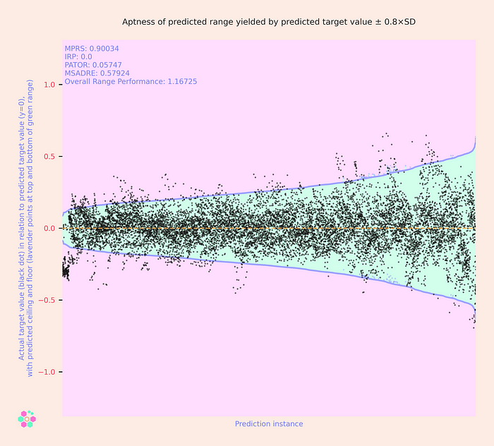

These display a characteristic funnel shape, with the only difference between models being the funnel’s amplitude. By choosing a smaller SD multiplier, it’s possible to create narrower (and potentially more managerially useful) prediction intervals for all workers — but at the cost of increasing the share of actual target values that will exceed their predicted ceiling or fall below their predicted floor. These models’ ORP is 1.16725 and 1.10903, respectively.
Now we can look at a selection of the joint range models fashioned from ANN-based ceiling and floor models employing custom loss functions. First is a model whose ceiling uses the loss function:
from keras import backend as K
loss = K.mean(math_ops.squared_difference(y_pred, y_true), axis=-1) \
    + 0.7 * K.mean(y_true - y_pred)
And whose floor utilizes the loss function:
loss = K.mean(math_ops.squared_difference(y_pred, y_true), axis=-1) \
    - 1.1 * K.mean(y_true - y_pred)
We see that this model manages to generate prediction intervals that contain the actual target values in the overwhelming majority of cases — but only by setting ceiling values that are generally quite high and floor values that are generally quite low. The sizes of the prediction intervals are relatively consistent across all workers. This model has an ORP of 1.06253, which is better than the MAE-based model but inferior to both of the SD-based models.
Next, we can look at the joint range model whose ceiling uses the loss function:
loss = K.mean(math_ops.squared_difference(y_pred, y_true), axis=-1) \
    + 0.55 * K.mean(y_true - y_pred)
And whose floor utilizes the loss function:
loss = K.mean(math_ops.squared_difference(y_pred, y_true), axis=-1) \
    - 0.85 * K.mean(y_true - y_pred)
We can see that this model displays greater flexibility and variety between workers when predicting their performance floors than when predicting their performance ceilings. Its ORP of 1.13988 is enough to surpass the MAE-based model and the model based on ± 0.8×SD, but it doesn’t match the effectiveness of the model based on ± 1.0×SD.
Finally, we can look at the model whose ceiling uses the loss function:
loss_pred_safely_high = K.square(y_pred - y_true)
loss_pred_too_low = 200.0 * K.square(y_pred - y_true)
loss = K.switch(
    K.greater_equal(y_pred, y_true),
    loss_pred_safely_high,
    loss_pred_too_low
    )
And whose floor utilizes the loss function:
loss = K.mean(math_ops.squared_difference(y_pred, y_true), axis=-1) \
    - 0.5 * K.mean(y_true - y_pred)
This model’s ORP of 1.27719 is the best of all 35 joint range models validated on the given dataset. The model manages to maintain relatively narrow prediction intervals for most workers, expanding only as much as is needed to accommodate the cases of workers whose 30-day mean efficacy scores are difficult to predict with much exactness.
More broadly, the 14 best-performing joint range models were all ones based on ANNs with custom loss functions; the best-performing “conventional” model (in 15th place) was the model based on ± 0.8×SD shown above. The MAE-based model was the worst-performing of the 35 joint range models.
Concluding the series
Of course, during this series of articles, we’ve only considered one particular forecasting assignment in HR predictive analytics as an example. It’s undoubtedly true that there are many kinds of assignments relating to the prediction of workers’ future job performance for which simpler MAE- or SD-based prediction intervals will generate superior results (and with much lower demand for computational resources). However, our analysis has illustrated that there are at least some situations in which the separate modelling of ceilings and floors through the use of ANNs with custom loss functions — while being somewhat more complex — possesses the potential to generate more accurate, nuanced, and useful forecasts, when it comes to predicting the likely range of a worker’s future performance. Through such approaches, it may be feasible to supply managers with prediction intervals that are as narrow (and thus meaningful) as possible, while still being wide enough to include all potential results that a worker might reasonably be expected to generate.
Having explored the usefulness of such independently-modelled prediction intervals, it will be easier to recognize particular scenarios in which such kinds of machine learning may be appropriate in one’s daily work in HR predictive analytics. Thank you for your engagement with this series!
